


- 29 JANUARY 2024 · RESEARCH BULLETIN NO. 115
Quantifying financial stability risks for monetary policy
When inflationary pressures started intensifying in 2022, the world’s major central banks faced a dilemma. They could rapidly tighten monetary policy at the risk of fuelling financial distress after years of ultra-low interest rates and balance sheet expansion, potentially amplifying the intended effects of the policy move on the real economy and inflation. Or they could take a more gradual approach to fighting inflation that would protect the financial system, but risk high inflation becoming entrenched. While severe financial instability may be an unlikely event (or “tail risk”), it can have devastating macroeconomic consequences. Quantifying financial stability trade-offs therefore requires a way to gauge the three-way interaction between monetary policy, financial stability conditions and tail risks to the economy.
Assessing tail risks to the euro area economy
In Chavleishvili, Kremer and Lund-Thomsen (2023), we develop a novel approach to gauge the potential short- to medium-term costs and benefits of alternative policy actions when monetary policy faces trade-offs between financial and macroeconomic stability. The structural quantile vector autoregressive (QVAR) model – introduced by Chavleishvili and Manganelli (2023) – provides a flexible way of estimating the dynamic interactions between our main variables of interest: real GDP growth, inflation, short-term interest rates and financial stability conditions.[2] The “flexible” attribute refers to the fact that the estimated interactions can be weaker or stronger in the centre and in the tails of the “joint probability distributions” of the model variables. Financial stability conditions are captured by two summary indicators measuring financial imbalances and system-wide financial stress, respectively. Using quantile regression allows us to uncover non-linearities in the dynamics of the model variables like in the seminal “growth-at-risk” paper by Adrian et al. (2019), which documents a much stronger impact of financial distress on the left tail of the growth distribution. By considering the entire probability distribution of our variables of interest, we can evaluate policy options not just in terms of their most likely outcomes, but also in terms of the tail risks associated with particularly undesirable states such as systemic crises. The quantification of tail risks thus lends itself to a risk management perspective on financial stability considerations in monetary policy (see Kilian and Manganelli, 2008), a perspective that focuses on the balance of upside and downside risks to inflation and economic activity rather than on the mean forecasts of both variables.
To operationalise financial stability, our model includes two measures widely used in ECB analysis. The first one is the Systemic Risk Indicator (SRI), which measures the financial cycle and, by extension, system-wide financial imbalances (see Lang et al., 2019). The second is the Composite Indicator of Systemic Stress (CISS), which quantifies systemic stress in the financial system (see Holló et al., 2012, and Chavleishvili and Kremer, 2023). Conceptually, one may think of the former as systemic risk ex ante, i.e. the risk of a future financial crisis, and of the latter as systemic risk ex post, i.e. materialised systemic risk. A typical financial boom-bust cycle would then see an elevated level of the SRI followed by a steep rise in the CISS as the bubble bursts and the system deleverages, with the Great Financial Crisis being a prominent example. The risk of such a boom-bust pattern poses an intertemporal financial stability trade-off for monetary policy: it can try to curb the financial boom by keeping interest rates higher than they would otherwise be, at the cost of weaker economic growth over the short run and at the benefit of a financial crisis being less likely and less severe over the medium term. In this article, however, we focus on another: the intratemporal financial stability trade-off for monetary policy, in which monetary policy itself may trigger more immediate financial instability.
The intratemporal financial stability trade-off in 2022
The circumstances prevailing in 2022 in the euro area and in many other places in the world, marked a stark turning point in the monetary policy stance. At the time, surging inflation called for a sharp tightening of monetary policy, even though economic growth was slowing after the post-pandemic rebound and financial stress was increasing on the back of the Russian aggression in Ukraine. In addition, the financial system at the time was vulnerable to a policy reversal because after a decade of accommodative monetary policy, the yield curve was flat and risk premia were at historically low levels, implying elevated risks to the profitability of banks and other financial intermediaries from a sharp rise in short-term interest rates.
To quantify the intratemporal financial stability trade-off in the euro area, we forecast the full distribution of our model variables over a period of four years, starting with the fourth quarter of 2022 (Q4 2022). In the baseline scenario, we fix the path of interest rates to the expected short-term market rates from the September 2022 Survey of Monetary Analysts (SMA) conducted by the ECB. In the baseline, we also require the mean forecast of real GDP growth, HICP inflation and commodity prices between Q4 2022 and Q4 2024 to reflect the ECB's publicly available macroeconomic projections. This approach allows us to replicate the context in which policymakers were deciding on the path forward at the time while still considering macro-financial tail risks.
In addition to the baseline scenario, we also consider two alternative policy scenarios with different paths of short-term interest rates. The first one is “front-loading”, whereby policy rates are hiked more quickly. This helps prevent inflation from becoming entrenched, but it can also hurt systemically relevant banks and other financial intermediaries that have become particularly vulnerable to interest rate risk. The March 2023 banking turmoil in the United States and elsewhere provides a clear example of how monetary tightening may induce, or expose, financial fragility (see, e.g., Jiang et al., 2023, and Acharya et al., 2023). The second scenario considers a gradual monetary tightening. This may alleviate strains on financial stability, but at the cost of making high inflation more persistent, thereby creating the risk of long-term inflation expectations becoming de-anchored from the ECB’s 2% target. All three interest rate paths are illustrated in Chart 1.
Chart 1
Counterfactual paths for short-term interest rates in the euro area
Pct. p.a.
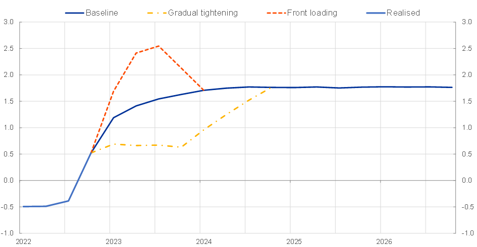
Sources: ECB, LSEG and authors’ calculations.
Notes: We use the three-month euro area overnight index swap (OIS) rate to capture short-term interest rates in our model. “Gradual tightening” considers an interest rate path in which the interest rate hikes in Q4 2022, Q1 2023 and Q2 2023-Q3 2023 are 50 basis points, 25 basis points, and 12.5 basis points lower than the baseline path. The gap to the baseline is then linearly closed over the subsequent four quarters. “Front loading” considers a path where interest rates are raised by an additional 50 basis points in Q4 2022 and Q1 2023 compared to the baseline, after which the gap is closed over the period Q3 2023-Q4 2023. In both cases, the initial deviation from the baseline path thus totals 100 basis points.
Chart 2 plots the projected paths of the mean as well as the 10th and 90th percentiles of the forecast density of real GDP growth and the CISS using the three interest rate paths above. As previously noted, in the case of real GDP growth, the dotted line is restricted to meet the ECB’s growth projections at the time. The 10th and the 90th conditional percentiles represent the downside and the upside tail risks around these mean projections, respectively.[3] Looking at the chart, we see that downside risks to real GDP growth (blue lines, left chart), as well as upside risks to systemic stress (red lines, right chart) are amplified by the interest rate front-loading in the short term compared to the baseline, and that the effects are larger compared to the respective opposite tails. Tightening monetary policy above market expectations increases the probability of realising a high level of systemic stress, in turn feeding into downside risks to growth. In contrast, a more gradual tightening has the opposite effects.
Chart 2
Forecast distributions of euro area real GDP (left) growth and the CISS (right) in the three policy scenarios
Real GDP Growth | CISS |
Pct., year-on-year | Pure number |
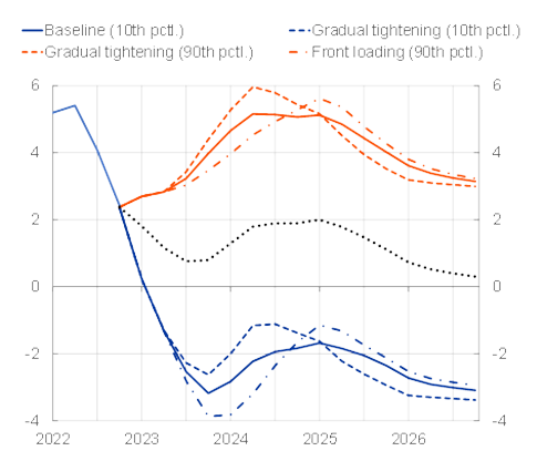 |  |
Sources: ECB and authors’ calculations.
Notes: For real GDP growth, the mean baseline projection equals the ECB staff projection from September 2022 up to and including Q4 2024.
Overall, when comparing the short- to medium-term costs and benefits of the scenarios vis-à-vis the baseline forecast, the results generally do not support a more aggressive tightening path than what was expected by market participants in the autumn of 2022. The elevated downside risks to growth may outweigh the only modest gains in lower predicted inflation. That said, a policymaker who is particularly concerned about inflation expectations becoming de-anchored from target inflation may still be inclined to favour tighter policy. On the other hand, if policymakers were more concerned about the risk of causing severe financial distress by front-loading policy, the scenario could be modified to resemble, for example, the so-called “taper tantrum”, an episode of severe financial stress that occurred in 2013 when the Federal Reserve hinted at tapering its bond-buying programme.
Another consideration is that we have modelled monetary policy rather simplistically, with short-term rates being the only instrument. Today, monetary policymakers have several tools available, some of which can be used to separately target price and financial stability concerns, potentially mitigating the intratemporal financial stability trade-off. Still, a policymaker may prefer to avoid sparking financial stress to begin with, even if it can be contained with the right combination of tools.
Monetary policy from a risk manager’s perspective
In this article, we sketched a novel empirical approach to quantify the macroeconomic costs and benefits of monetary policies which take financial stability considerations explicitly into account. The approach has the distinct advantage that financial stability considerations are not introduced ad hoc or as pure “side effects” of monetary policy. In contrast, financial stability trade-offs enter the policy calculus through their direct effects on future inflation and economic activity. Our approach allows monetary policymakers to adopt a risk management perspective when confronted with elevated macroeconomic tails risks associated with certain risks to financial stability.
References
Acharya, V. V., Chauhan, R. S., Rajan, R. G., and Steffen, S. (2023), “Liquidity dependence and the waxing and waning of central bank balance sheets”, NBER Working Paper, No. 31050.
Adrian, T., Boyarchenko, N. and Giannone, D. (2019), Vulnerable growth. American Economic Review, Vol. 109(4), pp. 1263–89.
Chavleishvili, S. and Kremer, M. (2023), “Measuring systemic financial stress and its risks for growth”, Working Paper Series, No. 2842, ECB.
Chavleishvili, S., Kremer, M. and Lund-Thomsen, F. (2023), “Quantifying financial stability trade-offs for monetary policy: A quantile VAR approach”. Working Paper Series, No. 2833, ECB.
Chavleishvili, S. and Manganelli, S. (2023), “Forecasting and stress testing with quantile vector autoregression”, Journal of Applied Econometrics, forthcoming.
Holló, D., Kremer, M. and Lo Duca, M. (2012), “CISS - A composite indicator of systemic stress in the financial system”, Working Paper Series, No. 1426, ECB.
Jiang, E., Matvos, G., Piskorski, T., and Seru, A. (2023), “Monetary tightening and U.S. bank fragility in 2023: mark-to-market losses and uninsured depositor runs?” NBER Working Paper, No. 31048.
Kilian, L., and Manganelli, S. (2008), “The central banker as a risk manager: Estimating the Federal Reserve’s preferences under Greenspan”, Journal of Money, Credit and Banking, Vol. 40(6), pp.1103-29.
Lang, J. H., Izzo, C., Fahr, S. and Ruzicka, J. (2019). “Anticipating the bust: a new cyclical systemic risk indicator to assess the likelihood and severity of financial crises”, Occasional Paper Series, No. 219, ECB.
This article was written by Sulkhan Chavleishvili (Aarhus University), Manfred Kremer and Frederik Lund-Thomsen (both Directorate General Research, European Central Bank). It is based on the paper by the same authors titled “Quantifying financial stability trade-offs for monetary policy: a quantile VAR approach”, ECB Working Paper Series No. 2833. The authors gratefully acknowledge the comments of Ana Maria Borlescu, Gareth Budden, Alexander Popov and Zoë Sprokel. The views expressed here are those of the authors and do not necessarily represent the views of the European Central Bank or the Eurosystem.
We also include global commodity price inflation as a variable that captures one source of supply-side pressures on inflation.
The 10th to 90th percentile ranges reflect the width of the forecast distributions and should not be confused with confidence bands from standard statistical analysis.